Tutorials
Five short, complete walkthroughs with real inputs from the PDB and the output they produce. Commands assume sesmesh 1.1 on your PATH (cargo install sesmesh-cli), plus curl and jq.
PDB ID → picture
CLI · 10 minutes · haemoglobin (4HHB)
Download a structure
Any entry from the PDB works; mmCIF is the archive's native format. sesmesh reads it gzipped.
Shell$ curl -LO https://files.rcsb.org/download/4HHB.cif.gzLook before you mesh
infoshows models, chains, composition and whether the radius set covers every atom.Shell$ sesmesh info 4HHB.cif.gz chains: 4 (A:1168 B:1224 C:1171 D:1216) elements: C:2954 O:1027 N:780 S:12 Fe:4 P:2 hetero atoms: 395 hydrogens: 0 water atoms: 221 alt-loc atoms: 0 selected: 4558 atoms radii (bondi): 4554 of 4558 atoms covered, 4 fallback (1.80 Å)Mesh it
A fine grid for detail, internal cavities removed, colours by chain, then decimated to 30 % of the triangles — the kept vertices are still exactly on the surface.
Shell$ sesmesh 4HHB.cif.gz -q high --cavities remove \ --vertex-colors chain --decimate 0.3 -o 4hhb.plyOpen it
Binary PLY keeps positions, normals and colours compactly. Blender: File ▸ Import ▸ Stanford PLY, then in the material feed a Color Attribute node into Base Color. MeshLab and ParaView open it directly. For tools that prefer OBJ, write
-o 4hhb.obj(colours asv x y z r g b).Try other colourings
Shell# chemistry: the nearest atom's element (bundled palette, or --palette file.json) $ sesmesh 4HHB.cif.gz -q high --vertex-colors element -o 4hhb-el.ply # geometry: convex (contact), saddle (toroidal) and concave (re-entrant) patches $ sesmesh 4HHB.cif.gz -q high --vertex-colors patch -o 4hhb-patch.ply
Cavities & areas
CLI + jq + Python · 15 minutes · GroEL–GroES (1AON), haemoglobin (4HHB)
Keep only the cavities
The exact SES contains closed internal cavities with negative signed volume. Keep just them, drop the tiny ones, and record the numbers.
Shell$ sesmesh 1AON.cif.gz -q high --cavities only --min-cavity-volume 5 \ --group-components --stats cavities.json -o cavities.obj $ jq '[.components[] | select(.cavity)] | length' cavities.json 285 $ jq -c '.components[] | select(.cavity) | {index, volume, area}' cavities.json | head -3 {"index":0,"volume":-13.174403395890868,"area":27.0622199529793} {"index":1,"volume":-11.614457386530887,"area":24.868030910443903} {"index":2,"volume":-86.08582206107998,"area":128.0659578151871}Per-atom surface area
--atom-areaswrites the SES area of every selected atom: index, serial, chain, residue, atom name, element, radius, area.Shell$ sesmesh 4HHB.cif.gz -q high --atom-areas areas.csv -o /dev/null $ head -3 areas.csv atom,serial,chain,res_name,res_seq,ins_code,atom_name,element,radius,area 0,1,A,VAL,1,,N,N,1.550,16.8767Save as
residues.pyand sum per residue with nothing but the standard library:Pythonimport csv from collections import defaultdict area = defaultdict(float) with open("areas.csv") as f: for row in csv.DictReader(f): area[(row["chain"], row["res_name"], int(row["res_seq"]))] += float(row["area"]) for (chain, name, seq), a in sorted(area.items(), key=lambda kv: -kv[1])[:10]: print(f"{chain} {name}{seq}: {a:.1f} Ų")Shell$ python3 residues.py C HEM142: 217.9 Ų D HEM148: 214.8 Ų B HEM148: 211.8 Ų ...Buried interface area
The surface two chains lose when they meet: mesh each chain alone and together, then subtract.
Shell$ for c in A B A,B; do sesmesh 4HHB.cif.gz -q high --chains $c --no-hetatm --cavities remove \ --stats - -o /dev/null --quiet | jq .mesh.area done 7197.0 # A 7493.8 # B 13651.5 # A,B → buried: 7197.0 + 7493.8 − 13651.5 = 1039.3 Ų
A virus on a laptop
CLI · 10 minutes · dengue virus capsid (1K4R, assembly 1)
Find the assembly
Deposited coordinates are often one asymmetric unit. The biological assembly is built from the file's operators.
Shell$ curl -LO https://files.rcsb.org/download/1K4R.cif.gz $ sesmesh info 1K4R.cif.gz chains: 3 (A:3028 B:3028 C:3028) assemblies: 1 (60 copies), 2 (1 copy), 3 (5 copies), 4 (6 copies), 5 (1 copy)Mesh 545 040 atoms
The full dengue virus capsid at 1 Å: about 10 s and 9.9 million triangles on a 10-core laptop (about 6 s on an AMD Zen 5 16-core system), in under 2 GB of memory.
Shell$ sesmesh 1K4R.cif.gz --assembly 1 -q draft --progress --timings -o capsid.ply sesmesh: 4937664 vertices, 9883296 triangles, 1123 component(s) (1098 cavities), ...Make it viewer-friendly
Cap the triangle count and colour by chain; decimation keeps the surface exact where it keeps vertices.
Shell$ sesmesh 1K4R.cif.gz --assembly 1 -q draft --max-triangles 1500000 \ --vertex-colors chain -o capsid-1.5M.plySet a memory budget
Before any mesh exists, sesmesh estimates the peak memory of the whole run. With
--max-memoryalone, inputs whose estimate exceeds the limit stop with exit code 4. Add--auto-coarsento grow the spacing until the estimate fits; the spacing used and the estimate are printed, and the statistics JSON records them (engine.estimated_memory,engine.estimated_triangles).Shell$ sesmesh 1K4R.cif.gz --assembly 1 -q high --max-memory 1G --auto-coarsen \ --max-triangles 1500000 -o capsid.ply sesmesh: ... 545040 atoms (model 1), ses surface, probe 1.40 Å, grid 2.402 Å sesmesh: estimated peak memory 1008.2 MiB (limit 1024.0 MiB, about 1837964 triangles before decimation) sesmesh: 745560 vertices, 1500000 triangles, 979 component(s) (810 cavities), ...The estimate is deliberately conservative: this run peaked at about 0.65 GB against an estimate of 1008 MiB. The grid chosen and the estimate are the same on every run and for any thread count.Stop any time
Ctrl-C cancels within about 100 ms and exits with code 130.
Ambient occlusion
CLI + Python · 10 minutes · haemoglobin (4HHB)
Get aomesh and the script
Ambient occlusion darkens what little light reaches: pockets, clefts, the seams between chains. sesmesh does not compute it; aomesh, a separate program, bakes it into any OBJ afterwards, and
ses_ao.py(Python standard library only) runs the two in a row.Shell$ cargo install aomesh-cli # 0.4.0 or later $ curl -LO https://raw.githubusercontent.com/uvar-apps/sesmesh/main/tools/ao/ses_ao.pyMesh and bake
Options after
--go to sesmesh unchanged.--bake-colorsalso writes a PLY whose vertex colours are the chain colours times the AO.Shell$ python3 ses_ao.py 4HHB.cif.gz -o out --bake-colors \ -- -q high --vertex-colors chain --decimate 0.5 sesmesh: 320764 vertices, 641472 triangles, 33 component(s) (31 cavities), ... visibility min 0.000 mean 0.445 max 1.000 ses_ao: 4HHB.cif.gz: wrote 4HHB_ao.obj, 4HHB_ao.mtl, 4HHB_ao.png, 4HHB_ao.ply in out (sesmesh 1.19 s, aomesh 3.34 s, colours 1.42 s)What is in the files
4HHB_ao.objis the sesmesh surface unchanged (colours, normals, header) plus one texture coordinate per vertex, its AO value;4HHB_ao.mtlnames4HHB_ao.png, a 256 × 1 grey ramp from black (occluded) to white (open), as the diffuse map. Any renderer that draws textured OBJ shows the occlusion with no special support. The value is the cosine-weighted share of 256 viewpoints around the molecule that see the vertex:ao = (256·u − 0.5)/255from the coordinateu.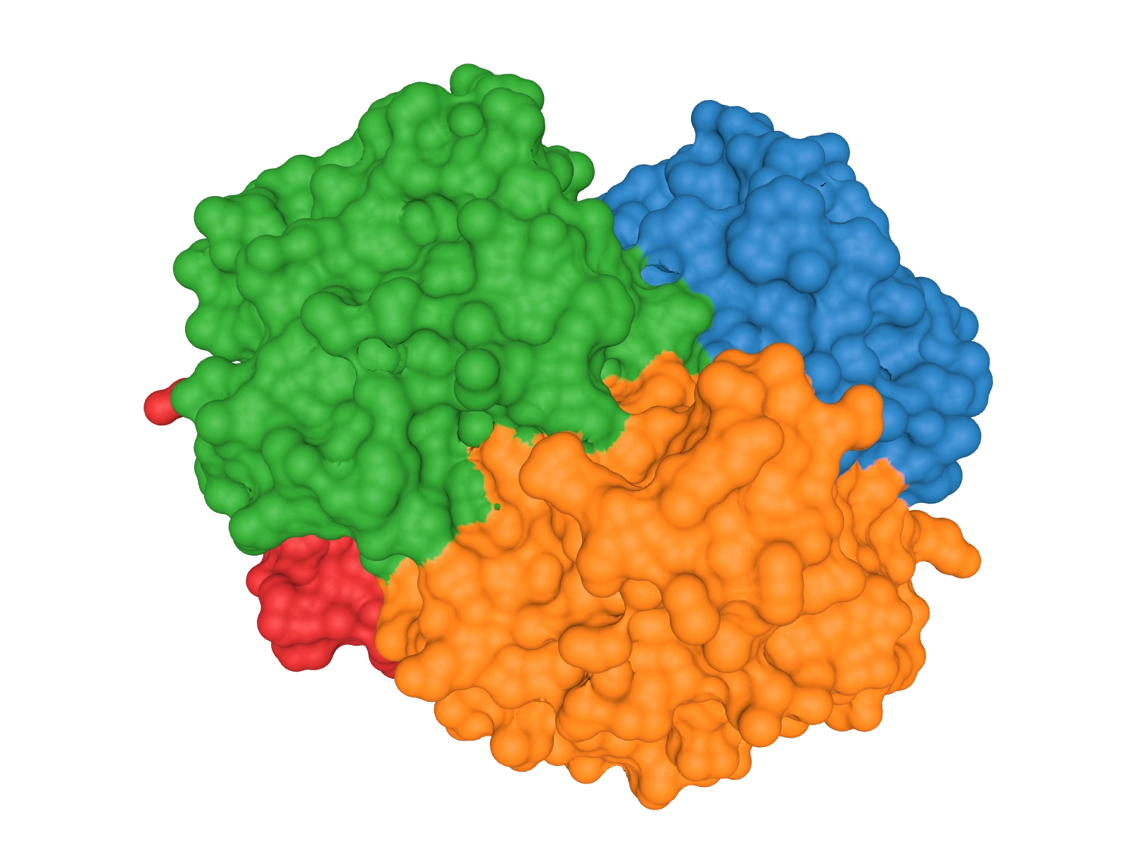 MISSING IMAGE
img/gallery/4hhb-chain.webpColoursThe surface as sesmesh writes it. 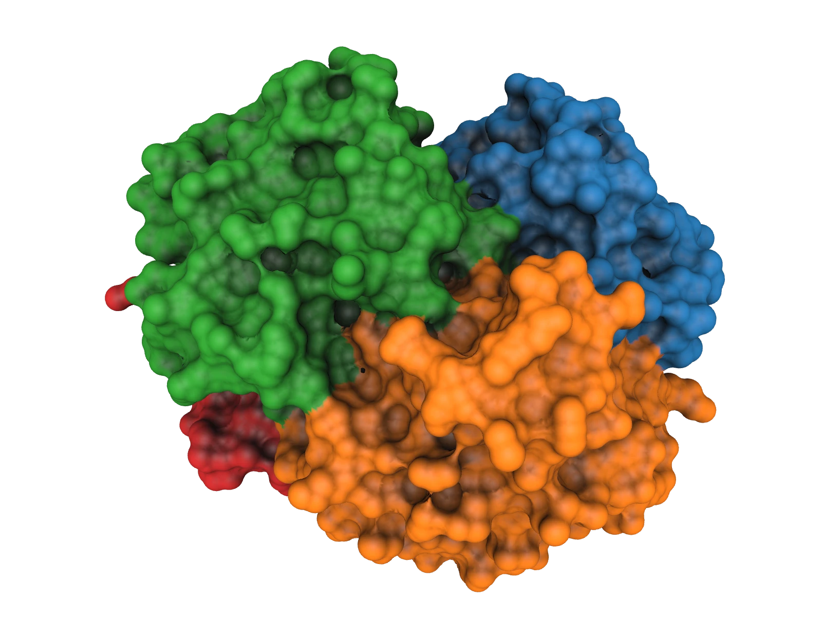 MISSING IMAGE
img/gallery/4hhb-chain-ao.webpColours × AOThe baked PLY: chain colours times the AO, same mesh and light. Open it
three.js:
MTLLoaderandOBJLoaderload the texture; turn on vertex colours to multiply the chain colours by the AO.JavaScriptimport { OBJLoader } from "three/addons/loaders/OBJLoader.js"; import { MTLLoader } from "three/addons/loaders/MTLLoader.js"; const materials = await new MTLLoader().loadAsync("out/4HHB_ao.mtl"); materials.preload(); const surface = await new OBJLoader().setMaterials(materials).loadAsync("out/4HHB_ao.obj"); surface.traverse((o) => { if (o.isMesh) o.material.vertexColors = true; }); scene.add(surface);Blender: File ▸ Import ▸ Wavefront (.obj) wires the ramp into Base Color; for colours × AO put a Mix node set to Multiply between the Color Attribute and the image texture, or import
4HHB_ao.plyand feed its Color Attribute to Base Color. MeshLab and ParaView: open the PLY.Scale it up
aomesh's time and memory grow with the vertex count: GroEL–GroES at 0.5 Å has 2.2 million vertices and took 32 s and 3.1 GB. Cap the triangles first, and drop the cavities, which no outside viewpoint sees and which therefore come out black.
Shell$ python3 ses_ao.py 1AON.cif.gz -o out --bake-colors \ -- -s 0.5 --cavities remove --vertex-colors chain --max-triangles 1000000All options, more examples and the viewer notes: tools/ao/README.md. A surface you already have is baked as is:python3 ses_ao.py surface.obj --samples 1024.
Trajectories in Rust
Rust · 15 minutes · Trp-cage NMR ensemble (1L2Y)
Create a project
Shell$ cargo new ensemble && cd ensemble $ cargo add sesmesh $ curl -LO https://files.rcsb.org/download/1L2Y.cif.gzCargo.toml[package] name = "ensemble" version = "0.1.0" edition = "2024" [dependencies] sesmesh = "1"Mesh every model
One
SurfaceEnginefor all frames: parameters are validated once and per-thread buffers are reused. Each model is selected withModelChoice::Index.src/main.rsuse sesmesh::io::{ReadOptions, read_path}; use sesmesh::radii::{RadiusOptions, assign}; use sesmesh::structure::ModelChoice; use sesmesh::{Diagnostics, Selection, Sphere, SurfaceEngine, SurfaceParams}; fn main() -> sesmesh::Result<()> { let path = std::env::args().nth(1).unwrap_or_else(|| "ensemble.pdb".into()); let structure = read_path(&path, &ReadOptions::default())?; let mut engine = SurfaceEngine::new(SurfaceParams::ses(1.4).with_spacing(0.4))?; println!("model,atoms,area_A2,volume_A3,components"); for index in 0..structure.models.len() { let mut selection = Selection::default(); selection.model = ModelChoice::Index(index); let mut diags = Diagnostics::new(); let atoms = structure.select(&selection, &mut diags)?; let radii = assign(&atoms, &RadiusOptions::default(), &mut diags)?; let out = engine.compute(&Sphere::from_atoms(&atoms, &radii)?)?; println!( "{},{},{:.2},{:.2},{}", index + 1, atoms.len(), out.stats.area, out.stats.volume, out.stats.components ); } Ok(()) }Run it
Shell$ cargo run --release -- 1L2Y.cif.gz > areas.csv $ head -4 areas.csv model,atoms,area_A2,volume_A3,components 1,154,1271.87,2064.42,1 2,154,1332.64,2037.91,1 3,154,1342.58,2045.66,1The Trp-cage NMR ensemble has 38 models; over the first five the SES area varies by about 8 %, the enclosed volume by 3 %.
Go further
Add
Controlfor progress bars and cancellation (engine.compute_with), write meshes per frame withexport::ply::write_ply_path, or query the exact field withSesField— see the library guide.